How to Optimize a Waveform
Last Updated on March 29, 2024 by ImageXpert Team
In our introductory article on inkjet waveforms, we described what a waveform is and how the process of applying it to the printhead works. Now we consider how to optimize that waveform to get better jetting, using a general dropwatcher approach that applies to many printheads. For those of you that have received a waveform from your printhead or ink supplier, you may be wondering whether waveform optimization is necessary and worth your time and effort. In some cases, a generic waveform that is not tuned for a particular ink or industry application is good enough, but in many cases it is not.
To help explain, rather than printing images, let’s consider the process of taking images. On your digital camera there are settings for white balance, exposure, shutter speed, etc to help control how the image is captured. The camera comes with a preset combination of settings that will work well for general use, and this is probably what most people use – just point and click. But when you want to shoot images at night, or on a sunny day, or of a person, or of a landscape, a professional photographer is able to manipulate the settings to get much better results for each of these very different scenarios. Inkjet waveforms are very similar – there is such a difference in requirements between printing a coating, a graphic, a circuit board, or a metal part that a generic combination of waveform settings won’t be able to perform well in all of them. Nobody knows your ink and application like you do, so we want to bring you up to professional status with the knowledge to tune a generic waveform to get optimal results for your exact application.
In this article, we will follow along step-by-step with a Dimatix Samba G3L printhead to give example images and data along the way.
QUICK REMINDER OF THE PRINCIPLES
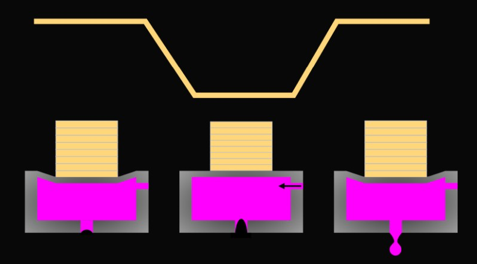
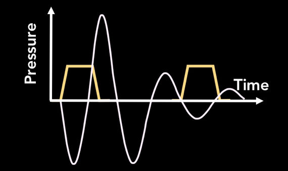
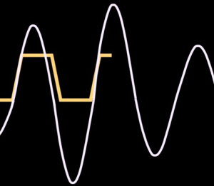
Let’s start by reviewing very briefly what we discussed in our other printhead and waveform articles. In the schematic below, we show how a voltage pulse results in deformation of the actuator, creating pressure in the nozzle chamber and causing a drop to eject. What we are optimizing is the size, shape, and spacing of the pulses to ensure that the jetting matches our target requirements.
UNDERSTANDING YOUR TARGET
The first step of any attempt to develop a waveform is to clearly define the goal. Usually, the most important targets to identify are the desired drop size, drop velocity, and jetting frequency. If you already know the target specifications, then you can get started straight away. If not, then you will have to do some investigation. Remember that different applications will have very different requirements for the jetting performance. Coating applications are primarily concerned with maximum throughput, and the stability at different speeds or number of satellites are of little concern. Contrast this to printed electronics, where printing consistency is everything. The printheads are very close to the surface, so slow drop velocities are acceptable, but no satellites and consistency in drop size across the printhead are crucial. Direct to shape applications have varying distances to the surface, so the drop speed and therefore throw distance should be maximized. 3D printing applications don’t want speeds that are too high (cause powder splash) or too low (won’t penetrate the powder). As you can see, you have to understand the needs of the application before beginning the process of tailoring a waveform to it.
If you are an ink company and have a specific machine to develop for, check with your customer what the usage conditions of the ink are. If your customer is an equipment manufacturer, they should be able to tell you all you need to know. If selling direct to user, then perhaps this information is not so easily available and you’ll have to work a bit harder to figure out what’s sensible.
One question that we are commonly asked is how to determine the necessary jetting frequency for your application. This is directly related to the printing resolution (in the process direction) and the carriage speed. In a simple example, let’s say you have one printhead printing at 600dpi and are printing in one pass at 100 inches per second. 600 dots per inch multiplied by 100 inches per second equals 60,000 dots per second – your jetting frequency! This equation gets a little more complicated when you print multiple passes or have multiple printheads. For example, if it took you two passes instead of one to print 600dpi, that means each pass is only 300dpi. Recalculating our frequency brings us to 30,000 dots per second. Instead of a single printhead, you had two printheads working together, that means each pass is really only 150dpi per head. Recalculating our frequency brings us to 15,000 dots per second for each head. With this basic knowledge, you can calculate how fast each printhead will be jetting on more and more complex machines to determine which frequency you should be optimizing your waveform for.
THE STARTING POINT
The very first step in waveform optimization is to establish a sensible baseline for our jetting so we can view it with the dropwatcher. If possible, an easy technique is to start with the printhead manufacturer-recommended, or default, single pulse waveform. As well as typical pulse timing, there will usually be some kind of calibration voltage (sometime called “label” voltage). Use this to start with as it should produce reasonable jetting. For our Dimatix Samba example, we are going to start with a waveform from the printhead user manual: a 26V amplitude pulse with a pulse width of 2.18us (including a 40V/us rise time).
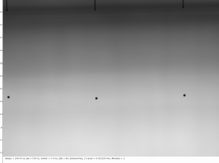
The next step is to get the drops visible in the field of view of the drop watcher. It is important that you can see the faceplate if possible; it helps a lot when it comes to understanding failures if you get them. The image below gives an ideal view for the Dimatix Samba printhead.
If you are just doing a preliminary test with a syringe fill, then it is useful to minimize the ink consumption during testing. Jetting about 10-20 nozzles along the same printhead row at a moderate frequency like 8kHz will allow you to test for a while without having to refill the fluid.
Do a quick measurement of the drop velocity to ensure that it is reasonable, maybe 5-6 m/s. Even if your eventual target is higher, this setting will usually allow easy measurements without too many satellites. If you find that the velocity is too low, you’ll want to increase the voltage of the pulse slightly, and vice versa. Our velocity happened to be acceptable without having to make modifications to the waveform, so 26V is an appropriate setting.
STEP 1: OPTIMIZING PULSE WIDTH
The first step in waveform optimization is to get the basic pulse shape to match the acoustics of the head and fluid combination. In waveform terminology, we will begin by determining the proper pulse width.
Because both the size of the nozzle and the fluid properties are fixed, we are looking for the amount of time to keep the nozzle chamber expanded that allows ink to move back and forth within it at a good rhythm.
In general, there is a near-quadratic relationship between pulse width and drop volume and velocity. The optimal pulse width is the one that will produce the highest drop volume and velocity, so finding that peak is what our first objective will be. Determine what the current pulse width is for your starting waveform, and plan to adjust the pulse width from 50% below to 50% above that recommended setting. At each pulse width, measure the drop volume and velocity at a consistent distance from the printhead. Choose a step size to give a few data points so you can build a curve.
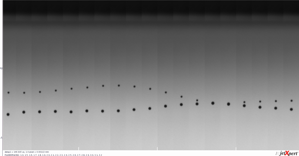
For our Samba printhead, we are going to automatically sweep through pulse widths from 1.1us to 3.3us in 0.1us increments. By capturing an image at each value (using double pulse) we are able to quickly judge the speed of the drop visually and can supplement with measurements if needed. The image below is generated using a combination of XSweep and Stitch.
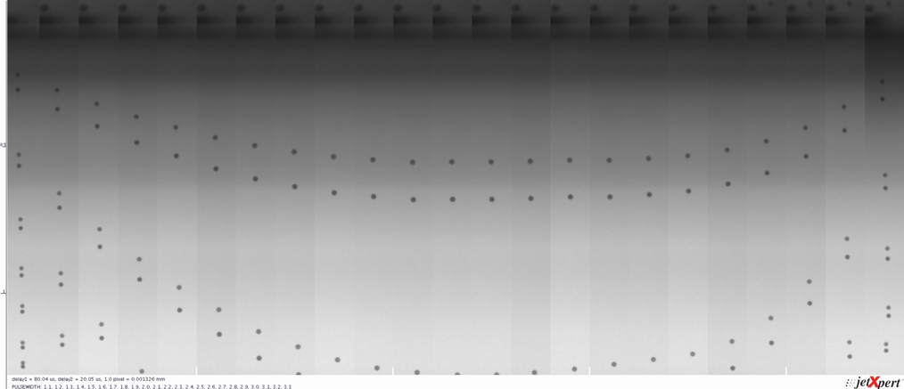
The top of the velocity curve is where the timing of the pulse gives the most efficient drop ejection for your combination of ink, head, and electronics. Sometimes it is desirable to use a pulse width a bit higher than the peak since it can help with satellites. Getting some experience will help you make this decision. Once you have selected your pulse width, program that value into your waveform and let’s continue forward.
Based on our image, we can see that pulse widths of 2.1-2.2us seem to produce the highest drop velocity. We can tell because each slice of the image was taken at the same moment in time, and the drop has travelled furthest from the printhead in these slices. If you recall, 2.18us was our starting pulse width from the Dimatix Samba manual, and indeed it seems to be optimal. Good job Dimatix!
SAVING TIME
As with most things in inkjet, it is up to the user to determine the level of precision to approach this process with. In the case of waveform optimization, choosing a smaller step size to test each parameter will be able to give you a more precise results. However, when doing this analysis manually, a smaller step size means the time it takes to do this testing increases. To make the process faster, ImageXpert has a tool called XSweep, which will automatically adjust the waveform settings and perform the measurements for you.
XSweep
Make the process of waveform optimization more automated with XSweep. Simply specify which waveform parameter you want to adjust, like voltage or pulse width, and a range of values to test, and the software will automatically capture images and data for each one.
See MoreSTEP 2: OPTIMIZING VOLTAGE
Now that we know we’ve got the timing right, we can explore the connection between voltage and drop volume and velocity. Usually, there is a linear relationship between voltage and drop volume and velocity, up to a limit. The normal trade-off is that increased voltage also produces increased ligaments, so the objective is getting the highest possible velocity that produces a nice clean drop without a tail that breaks into satellites.

As we did before with pulse width, let’s try a range of voltages and measure the drop velocity at each one. It is important to also keep an eye on the drop volume and satellite formation, as this will impact our decision. Our goal at this point is to determine the voltage setting that gives us our target volume and velocity without too many satellites. With our Samba, we are going to automatically sweep through voltages of 21V-31V in 0.5V increments. The output is shown below.
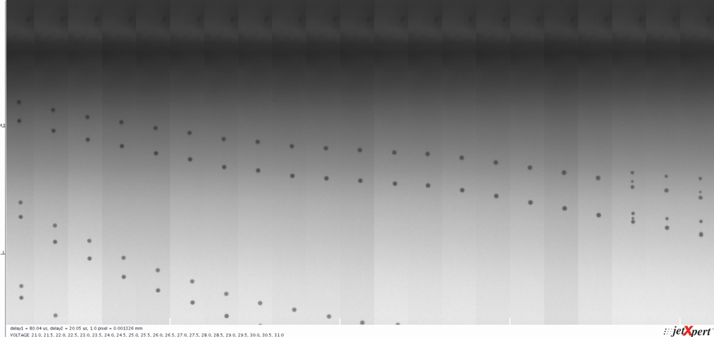
Once again, the results seem to match the theory. The drop velocity increases linearly with voltage, up to a point where satellites are introduced. Let’s choose a voltage a bit lower than the one that produced satellites and perform a measurement.
We now know the drop volume and velocity that a waveform using these settings will produce and can compare it to our targets. However, our job is not done yet.
Learning Something New? Subscribe to Receive Future Articles
STEP 3: PUSHING THE HEAD A BIT HARDER
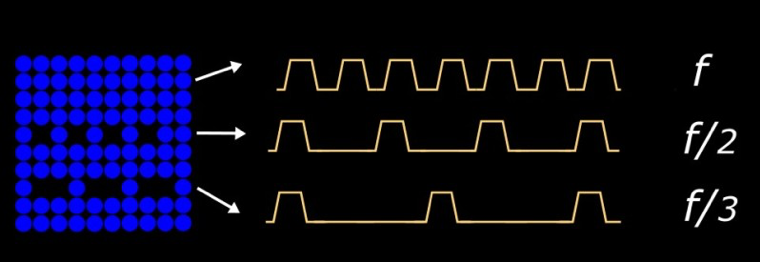
Now that you’ve improved your pulse and it’s producing the velocity you’ve been looking for, it is time to push the head a bit harder and turn up the frequency. This will test whether the waveform we’ve built so far performs well at our target frequency, as well as if there are any particular spots to avoid. If you already know what your key target frequency is, then you can save some time by just looking at jetting there, but don’t forget to include the subharmonics too. You may be surprised to learn that when an image is rendered and printed, the print resolution is not necessarily constant across the whole image. To help improve the appearance of the image, the resolution is increased for darker portions and decreased for lighter portions, making it possible to print a gradient even if you only have one available drop size. The resolution is commonly divided in half or in thirds, so testing one half and one third of your target frequency will ensure your waveform will still perform well after rendering.
We think it’s usually best to do as much as you can to understand the entire frequency space. You already have the system set up, and you never know when a customer will ask to use that ink at another frequency. In addition to XSweep, Imagexpert supplies the Frequency Sweep Add-On to help speed up the process. This will automatically sweep through a range of frequencies and collect the data, which is especially helpful for higher frequency printheads. The image below is our Samba waveform jetting at 1 – 30kHz in 1 kHz steps.
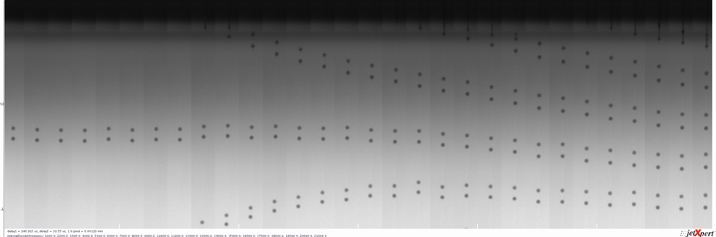
Fortunately, our drop formation looks pretty good across this range. Here is another example that tells a different story.
Notice how the jetting is a consistent velocity up until about 19 kHz, then the velocity spikes? In addition to the increased velocity, we also see increased ligament length and satellite formation. If you recall from our previous waveform article, this is resonance at work. At 19 – 24 kHz, the timing between the waveform pulses is such that the pulse is amplified by lingering momentum in the nozzle from pulse before it. With this knowledge, you can modify the design of your system to either avoid that frequency or use a different waveform for that range.
WHAT IF THE RESULTS ARE NOT GOOD?
If the waveform you’ve created does not perform well at the target frequencies, choose a lower voltage and try again. It is an iterative process, where you might need to make small changes to pulse width and voltage and repeat in order to get the results you want. This is where automation comes in handy. If you just can’t seem to get your drop volume or velocity high enough, multi-pulsing might be able to help.
STEP 4: INTRODUCING MULTI-PULSING
When more than one pulse is used in the waveform to create drops then we call it multi-pulsing. This is not to be confused with grayscale; we are still only producing one drop size, we are just using multiple waveform pulses to do it. Multi-pulsing can be useful for increasing the volume of the jetted drops if a single pulse is not capable of ejecting enough ink.
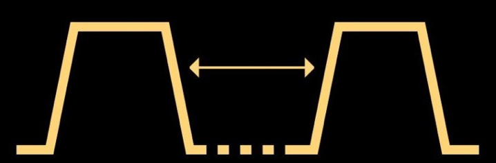
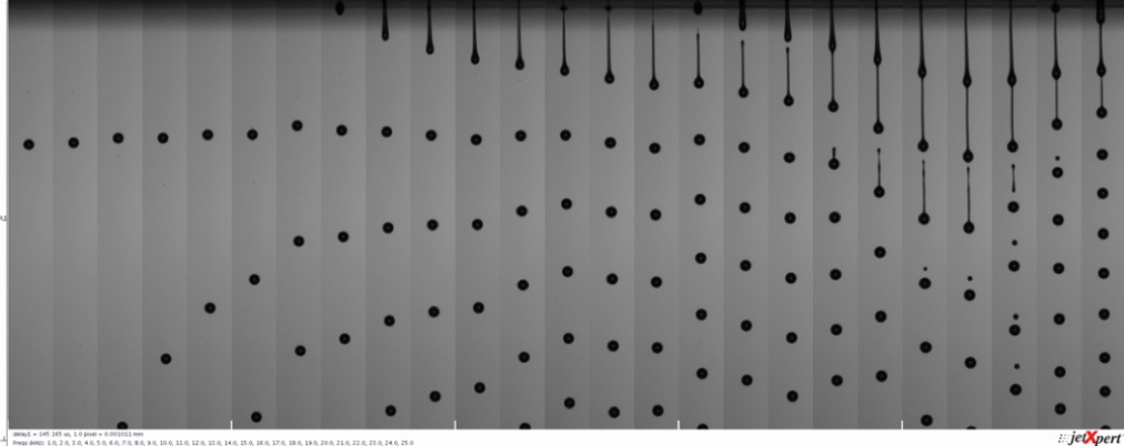
If we are going to use multiple pulses to create larger drops, we must begin by understanding the underlying timing of the ink moving in the head. We do this by creating two identical pulses and looking to see what happens to the ejection as function of the gap between them, as shown below. When the timing is right, the momentum of the ink in the nozzle will be increased by the second pulse, and we will see a faster drop once it is jetted.
Let’s duplicate the optimized pulse that we created from before and adjust the spacing between these two pulses, analysing the jetting at each step. A good starting point is to vary the spacing from the minimum allowable value to double the pulse width of each pulse. The best measurement to do is to look at the velocity of the second drop that comes out (if it does at all) since the speed of that drop is very sensitive to pressure fluctuation caused by the first pulse. At low pulse gaps in some head/ink combinations, the drops are likely to have merged before you get the chance to measure them, whilst in others the second ejection might appear as a bulge travelling up the ligament of the first. What is important is to find at what spacing the drop(s) you can measure go fastest. The peaks in the behaviour are where the head resonance lies. Most successful greyscale waveforms work on or near the resonance period so that the ejection is optimised for a given amount of input.
When we duplicated our optimized Samba pulse and swept the pulse spacing from 1.4us to 3.2us in 0.1us steps, we produced the following image. It is pretty clear where the speed of the second drop is the highest, which is our resonant period.

Now that we know our resonant period we can build a waveform that uses it. The only thing to remember is that if you are going to stack pulses like this one after another, it is important to consider the voltage amplitude or you’ll push that final ejection velocity really high. As we’ve discussed before, that usually is a bad thing for nozzle wetting and satellites. So, with that in mind, you may start with something like this to get your target drop size.
MAKING MULTI-PULSING DO GREYSCALE
As we mentioned already, the key difference with grayscale is having the ability to vary drop size at each pixel on the printed image. This means you need to choose which waveform pulses to use for each gray level to get the desired drop size. The first step to achieving this is to break the waveform into segments that can be selected by the print controller. You then must associate the right segments to the grey levels.
Just like the pulse shapes themselves, this part is very dependent on your system, and especially the software that allows you to edit the waveform “shape”. The easiest way to visualise this, and thus often used in patents on the subject, is to picture the waveform with separators and then have a table telling you which is used in each level. We have drawn this below for a single 5-pulse example.
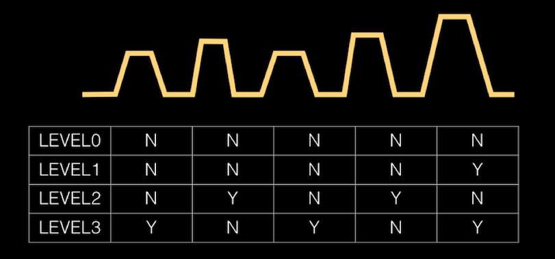
The reason we chose 5-pulse for 3 levels because it demonstrates nicely the high degree of flexibility that is possible, including the fact that pulse do not have to be identical or be linear in amplitude (like our first examples). The one thing to keep in mind is that the maximum frequency that can be used will be the inverse of the time taken to complete the whole waveform, regardless of which grey level you are selecting. For example, let’s say that you have three pulses in a waveform, each with a duration of 10us. Even if Gray Level 1 only uses a single 10us pulse, the maximum frequency that you can print at Gray Level 1 is based on 30us timing.
Usually there are rules associated to how close pulses can be to each other to allow time for the electronics board to switch between the waveform segments. Most good waveform editors will tell you if there’s a going to be a problem.
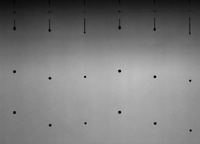
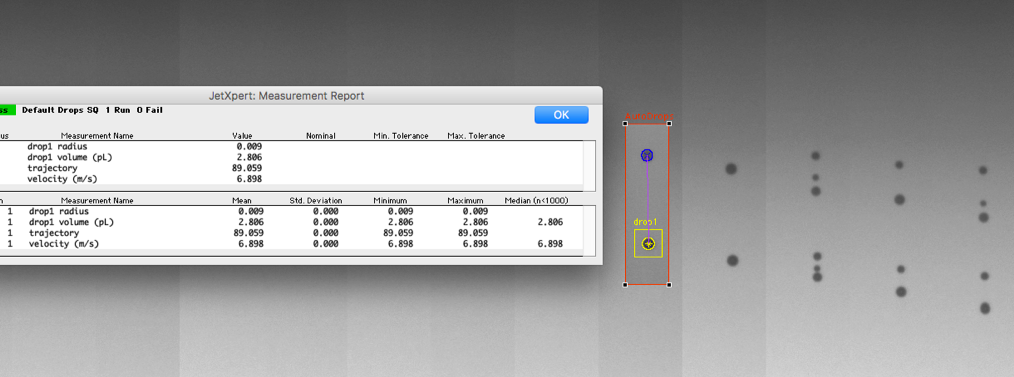
Now you can tune the individual pulse widths, voltages, and pulse spacings of the waveform segments to get the drop volume and velocity to match your targets. It is useful to have an image that places drops of different sizes next to each other in the same field of view, so you can study the impact of a change on all of the gray levels. This image shows three different gray levels in one field of view.
ADVANCED WAVEFORM DESIGN
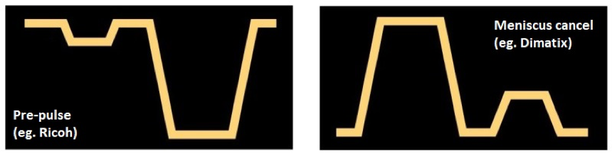
The multi-pulsing approach can also be useful for controlling nozzle plate wetting, or influencing ligament break-off, for example. Extra pulses can come before or after the main ejection pulse as shown below. Tips for implementing more advanced waveform tricks are hard to systematize but we wanted to make sure you know these things are possible. Two common types of pulses are pre-pulses and dampening / cancel pulses.
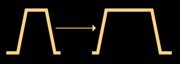
Pre-pulses are low amplitude pulses that come shortly before the main pulse, designed to help improve the efficiency of the ejection of the drop. They can help get the ink moving so that the ejection pulse has less energy to overcome (like rocking something before tipping it over). The timing of these pulses is critical to ensure that they are working with your main pulse and not against it!
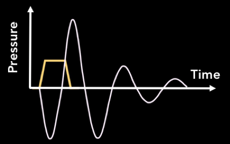
Dampening pulses are a similar concept but appear at the end of the waveform. After a pulse, there is some residual energy within the ink and it will continue moving inside the nozzle until it fades away. This can cause trouble at high frequencies, because the next cycle is starting while there is still movement in the nozzle, potentially leading to harmonic behavior. A perfectly-timed dampening pulse will work against the residual motion of the ink in the nozzle, bringing it to a stop. Reducing the oscillations of the ink in the nozzle may also have other benefits such as reducing wetting or shorter ligament length.
Slew rate is another term that you may have encountered in your waveform studies. The piezoelectric material that the nozzle walls are made from can only react so quickly, so there is a limit to the amount of voltage that you can apply to them in short intervals. The slew rate is the change in voltage over the change in time, almost like the acceleration of the walls. Printheads call for the sloping edges of the waveforms to fall within a certain range of slew rates for safe operation. Manipulating the slew rate may have some impact on the waveform and can be explored, but it is not nearly as noticeable as pulse width or voltage.
There is another method that is used by some head manufacturers as standard, called bi-polar pulsing. The terminology comes from heads that use both positive and negative amplifiers to drive the PZT in both directions. The advantage of such systems can be getting a more efficient drop ejection from a lower overall voltage, but it also allows pulses to be programmed in any direction for manipulating the pressure variation following ejection. Since bi-polar capability makes the electronics more complicated, the effect can be recreated using a uni-polar circuit (positive or negative voltage only) that uses a rest voltage that is non-zero. We try to explain the difference with the image below, which is taken from a couple of recent patents from two main head manufacturers. The image on the left is a bi-polar waveform, the image on the right is a uni-polar with a non-zero rest voltage.
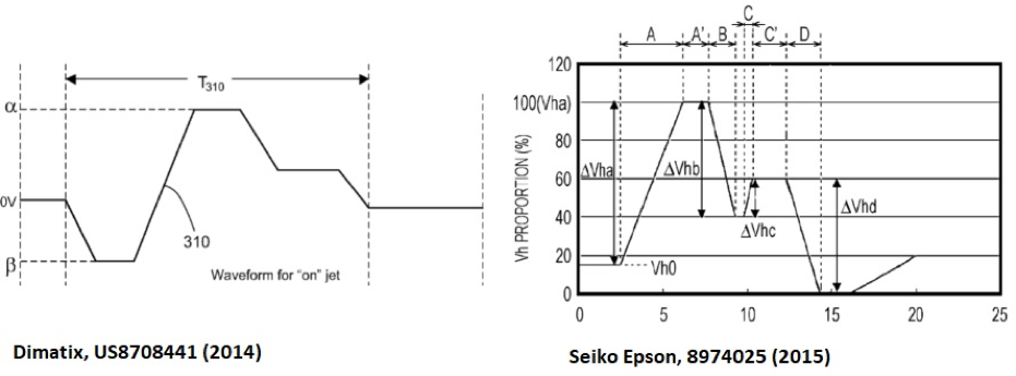
In both cases the waveforms are more than a succession of simple trapezoids like we described before. Generating the more arbitrary shapes needs a different approach than just how tall and wide the pulse will be. Usually the waveform is now defined by segments changing from one voltage to another over a given time. Some specific electronics are required and this can be vendor specific. Optimizing waveforms using these techniques may be elaborated on in a future article.
Referenced Products and Resources
-
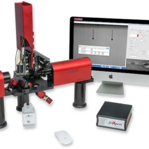
JetXpert Dropwatcher
Learn More -
What is a Waveform?
Learn More -
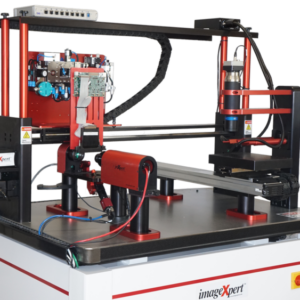
JetXpert Printers
Learn More